Math statistics - The science of how to systematize and use statistical data for scientific and applied purposes.

Mathematical statistics in psychology

In psychology as a science, mathematical statistics is used very widely. Using certain methods, for example testing, numbers are compared (scaled) to different features of human behavior, and these numbers are already worked with using the methods of mathematical statistics. After applying these methods, new data is obtained that should be interpreted.

Without the use of mathematical statistics, psychology would be a rather flat and uninformative science, based on conjecture and speculation (as is the case, for example, in psychoanalysis). Of course, the use of mathematical statistics is not an “antidote” against speculation and speculation, but the subject of discussion becomes much richer.

Let's consider a typical and simple case of using mathematical statistics. Let's say someone conducted a study of a group of schoolchildren. Among others, such parameters as extraversion-introversion and level of intelligence were found. The research psychologist was interested in how these parameters are related to each other. Is it true that introverts are, on average, smarter than extroverts? To do this, the group of subjects (sample) can be divided into two subgroups: extroverts and introverts. Next, for each subgroup, the arithmetic average for intelligence level is found. If, say, introverts have a higher IQ on average, then they are smarter than extroverts. This is one approach. Another might be to divide subjects into a subgroup with high IQ (over 100) and low IQ (less than 100), and then calculate the average for extraversion-introversion in each group. A third approach might be to use a more complex method, correlation analysis, instead of dividing into subgroups and calculating averages. All three of these methods are different, but will show the same connection.

Mathematical statistics allows you to make interesting, sometimes surprising discoveries. Let's continue with our hypothetical example. Suppose that a psychologist finds a paradoxical result that contradicts his past experience and knowledge. Let's say he found that in one school extroverts are smarter than introverts, although in all other schools it was the other way around. Why is that? A meticulous psychologist can begin his investigation and find that, for example, this is due to the fact that in this school extroverts go to the physics elective (because there is a “groovy teacher”) and develop their intelligence, and introverts go to the literature elective (because there is a “soul teacher”), where they develop other qualities of their soul. Can, for example, a psychoanalyst reach such a discovery? Highly unlikely.

In psychological research, not only purely psychological parameters such as, say, intelligence, extroversion or anxiety are taken into account. Data such as age, gender, education level, height, weight, physical strength, political views, work experience and much more can also be used. It often happens that without such non-psychological indicators, research turns out to be incomplete and uninformative. It also often happens that representatives of other sciences (for example, sociology or biology) also use psychological parameters in their research.

Mathematical statistics allows many things:

Practical psychologists in their work usually limit themselves to finding the arithmetic mean, divided into subgroups (as in the example above). Psychologists use a wide variety of mathematical statistics methods. Let's look at the main ones.

Finding the arithmetic mean

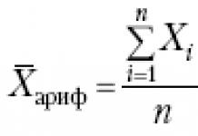
The most banal and simple method. Indicators (for example, the height of the subjects) are added up and then divided by the number of subjects. Despite its simplicity, the method is, of course, very informative and visual. Visualization is an important quality of the method for a practical psychologist. When he presents the results of his research to the customer (for example, the director of a school), he is not always able to understand the essence of correlation or variance analysis. Dividing subjects into subgroups based on an arbitrary basis enhances the potential of the arithmetic mean, making it possible to cover most of the researcher’s needs.

Finding the mode and median

Suppose we examined 1000 students and measured their height to the nearest centimeter. These data were entered into a table. If the most common value in the table is, say, 172 centimeters, this is fashion our sample. By the way, the word “fashion” is used in a similar way in everyday life: if this season you most often see red hats, then this means fashion, although the share of these hats may account for only 20 or 30 percent.

In psychological studies, the mode is usually somewhere around the arithmetic mean. If the fashion is 172 cm, then the average will be about that. The larger the sample, the closer the mode and the arithmetic mean.

Further. Suppose we divided our students into two equal groups: in the first group there are 500 short students, in the second group there are 500 high students. The growth value that falls on the 500th or 501st student is median. The median is usually also close to the arithmetic mean.

Detection of scattered values

As you know, the average temperature in a hospital is not that important. And in a good hospital, where they treat well, the average temperature can be 36.6°C; and in a bad situation it can be the same: just someone has a fever of 40°C, and someone has already died and has 18°C.

The easiest way to estimate sample dispersion is to find it scope(otherwise – scatter). If in our sample the shortest student is 148 cm tall, and the tallest is 205 cm, then the sample range will be 205-148 = 57 cm. This value is important primarily in order to assess the extent to which this parameter generally changes.

Further. Let's assume this situation. In twenty years, at the whim of some rich man, he will have clone children. In another twenty years they will go to university. And at the university there will be a sample of students of 1000 people, of which 998 have a height of 177 cm, one is 148 cm, one is 205 cm. In terms of the main parameters - arithmetic mean, mode, median, range - this sample may not differ from another sample of students (the same values ​​will be there). But at the same time, in the second (normal) sample there will be a certain number of students with a height of 150-160 cm, some with a height of 180-190 cm, etc. So, it turns out that from the point of view of mathematical statistics these groups are the same?

One glance at this figure is enough to understand that the groups differ in the dispersion of values. Therefore, in statistics there is a more accurate tool for estimating dispersion - dispersion. Dispersion is calculated as follows: find the arithmetic mean, then find the deviation from the mean for each case, square this value, and finally divide by the total number of cases. From the variance value it is easy to obtain standard deviation: it is the square root of the variance. Standard deviation stands for, understandably, standard deviation: that is, a measure of how much on average the values ​​deviate at all.

Standard deviation is measured in the same units as the parameter itself. In our first hypothetical group, where almost all students are the same, the standard deviation will be extremely small (less than 1 cm). In the second group there will be much more - 10-15 centimeters. If we are told that the average height of students is 175 cm with a standard deviation of 12 cm, we will know that the majority of students (about 2/3) are in the range of 163 to 187 cm.

Student's t-test

Suppose we decide to conduct an experiment of this kind. We took a group of subjects. Before the experiment began, they were tested, say, on their level of creativity. Then they spent a whole month drawing for an hour a day. At the end of the experiment, we again tested them for their level of creativity. A result was noticed, but quite small, and skeptics began to tell us that the level of creativity had not increased, a slight increase in the arithmetic average was just an accident.

For such situations, different criteria have been invented. One of them - the most popular - is the Student's t-test. In the numerator it has the difference of arithmetic means. The denominator is the root of the sum of squared variances (meaning the first and second testing cases). The greater the difference between the arithmetic means, the better (our work was not in vain), and the smaller the spread of values ​​in both diagnostic cases, the better: when the spread of values ​​is greater, then the random fluctuations are also greater.

To apply this criterion there is a significant limitation - the distribution of indicators should be close to the so-called normal(bell-shaped).

There are special criteria for determining the degree of normality of the distribution.

Correlation

In psychology, as probably in no other science, they like to find correlation coefficients. There are several different approaches, including both for normal and non-normal distributions. All of them show the degree of dependence of one parameter on another. If one parameter (for example, a person's weight) is highly dependent on another parameter (for example, a person's height), then the correlation coefficient will be close to +1. If the relationship is inverse (for example, the taller a person is, the less dexterous he is), then the correlation coefficient will tend to -1. If there is no dependence (say, luck when playing cards does not depend on a person’s height), then the correlation coefficient will be about 0.

If you take a group of subjects, record their height and weight, and then transfer the results to a two-dimensional graph, you will get something like the following picture, which indicates that the correlation is positive, approximately at the level of +0.5.

Factor analysis

Perhaps the most mysterious analysis. Some of its mystery is explained by the fact that it itself is intended to find a new parameter that explains a lot, but was not directly studied during the experiment. As a rule, during factor analysis the most influential parameters are found, on which smaller, more specific ones depend.

Let's say we conducted a study with schoolchildren. Among others, the following parameters were recorded: general academic performance, academic performance in science subjects, academic performance in humanities subjects, short-term memory capacity, volume and distribution of attention, mental activity, spatial imagination, general awareness, sociability, and anxiety. If you apply correlation analysis and create a so-called correlation matrix (which reflects the relationship of each parameter with each), you can see that most of these parameters correlate well with each other. The exception is the last two, which are weakly related to the others. Just looking at this matrix, we can assume that behind most of the parameters there is one common (super-parameter) that affects them all. We carry out the factor analysis procedure, and after that another column appears in our matrix - a column without a name. This mysterious parameter correlates very well with everything (except sociability and anxiety). After some creative thought, the psychologist comes to the only possible interpretation here - the mysterious parameter is intelligence. It influences everything else, its influence is strong, although not one hundred percent.

There are factor analysis methods that help identify not one, but several factors that influence other parameters. It often happens, of course, that a mysterious parameter turns out to be not so mysterious, but completely coincides with one of the parameters that were recorded. But sometimes it happens that you have to rack your brains for a long time before you can interpret this secret factor.

Factor analysis is used mainly by scientists to gain a deep understanding of the subject of research. It should be taken into account that for the accuracy of the result a fairly large number of subjects is necessary: ​​it is desirable that the number of subjects be several times greater than the number of parameters.

Using factor analysis, you can study the quality of psychological tests. If you take, for example, some personality questionnaire with several parameters, and subject these parameters to factor analysis, then some strange common factor may emerge that influences all parameters. It may not have a significant psychological meaning - it is simply the tendency of the subject to answer one way or another on a formal basis (someone answers thoughtfully, some are inclined to choose the first points from the options, some the last). The large influence of this general factor may indicate insufficient quality of assignments.

Literature

Ermolaev O. Yu. Mathematical statistics for psychologists: Textbook. - 2nd ed. corr. - M.: MPSI, Flinta, 2003. - 336 p.

RANDOM VARIABLES AND THE LAWS OF THEIR DISTRIBUTION.

Random They call a quantity that takes values ​​depending on a combination of random circumstances. Distinguish discrete and random continuous quantities.

Discrete A quantity is called if it takes on a countable set of values. ( Example: the number of patients at a doctor's appointment, the number of letters on a page, the number of molecules in a given volume).

Continuous is a quantity that can take values ​​within a certain interval. ( Example: air temperature, body weight, human height, etc.)

Law of distribution A random variable is a set of possible values ​​of this variable and, corresponding to these values, probabilities (or frequencies of occurrence).

EXAMPLE:

x	x 1	x 2	x 3	x 4	...	x n
p	p 1	p 2	p 3	p 4	...	p n

x	x 1	x 2	x 3	x 4	...	x n
m	m 1	m 2	m 3	m 4	...	m n

NUMERICAL CHARACTERISTICS OF RANDOM VARIABLES.

In many cases, along with the distribution of a random variable or instead of it, information about these quantities can be provided by numerical parameters called numerical characteristics of a random variable . The most common of them:

1 .Expected value - (average value) of a random variable is the sum of the products of all its possible values ​​and the probabilities of these values:

2 .Dispersion random variable:

3 .Standard deviation :

“THREE SIGMA” rule - if a random variable is distributed according to a normal law, then the deviation of this value from the average value in absolute value does not exceed three times the standard deviation

GAUSS LAW – NORMAL DISTRIBUTION LAW

Often there are quantities distributed over normal law (Gauss's law). main feature : it is the limiting law to which other laws of distribution approach.

A random variable is distributed according to the normal law if it probability density has the form:

M(X)- mathematical expectation of a random variable;

s- standard deviation.

Probability Density(distribution function) shows how the probability assigned to an interval changes dx random variable, depending on the value of the variable itself:

BASIC CONCEPTS OF MATHEMATICAL STATISTICS

Math statistics- a branch of applied mathematics directly adjacent to probability theory. The main difference between mathematical statistics and probability theory is that mathematical statistics does not consider actions on distribution laws and numerical characteristics of random variables, but approximate methods for finding these laws and numerical characteristics based on the results of experiments.

Basic concepts mathematical statistics are:

1. General population;

2. sample;

3. variation series;

4. fashion;

5. median;

6. percentile,

7. frequency range,

8. bar chart.

Population- a large statistical population from which part of the objects for research is selected

(Example: the entire population of the region, university students of a given city, etc.)

Sample (sample population)- a set of objects selected from the general population.

Variation series- statistical distribution consisting of variants (values ​​of a random variable) and their corresponding frequencies.

Example:

X,kg

m

x- value of a random variable (mass of girls aged 10 years);

m- frequency of occurrence.

Fashion– the value of the random variable that corresponds to the highest frequency of occurrence. (In the example above, the fashion corresponds to the value 24 kg, it is more common than others: m = 20).

Median– the value of a random variable that divides the distribution in half: half of the values ​​are located to the right of the median, half (no more) to the left.

Example:

1, 1, 1, 1, 1. 1, 2, 2, 2, 3 , 3, 4, 4, 5, 5, 5, 5, 6, 6, 7 , 7, 7, 7, 7, 7, 8, 8, 8, 8, 8 , 8, 9, 9, 9, 10, 10, 10, 10, 10, 10

In the example we observe 40 values ​​of a random variable. All values ​​are arranged in ascending order, taking into account the frequency of their occurrence. You can see that to the right of the highlighted value 7 are 20 (half) of the 40 values. Therefore, 7 is the median.

To characterize the scatter, we will find values ​​not higher than 25 and 75% of the measurement results. These values ​​are called 25th and 75th percentiles . If the median divides the distribution in half, then the 25th and 75th percentiles are cut off by a quarter. (The median itself, by the way, can be considered the 50th percentile.) As can be seen from the example, the 25th and 75th percentiles are equal to 3 and 8, respectively.

Use discrete (point) statistical distribution and continuous (interval) statistical distribution.

For clarity, statistical distributions are depicted graphically in the form frequency range or - histograms .

Frequency polygon- a broken line, the segments of which connect points with coordinates ( x 1 ,m 1), (x 2 ,m 2), ..., or for relative frequency polygon – with coordinates ( x 1 ,р * 1), (x 2 ,р ​​* 2), ...(Fig.1).

m m i /n f(x)

Fig.1 Fig.2

Frequency histogram- a set of adjacent rectangles built on one straight line (Fig. 2), the bases of the rectangles are the same and equal dx , and the heights are equal to the ratio of frequency to dx , or R * To dx (probability density).

Example:

x, kg	2,7	2,8	2,9	3,0	3,1	3,2	3,3	3,4	3,5	3,6	3,7	3,8	3,9	4,0	4,1	4,2	4,3	4,4
m

Frequency polygon

The ratio of relative frequency to interval width is called probability density f(x)=m i / n dx = p* i / dx

An example of constructing a histogram .

Let's use the data from the previous example.

1. Calculation of the number of class intervals

Where n - number of observations. In our case n = 100 . Hence:

2. Calculation of interval width dx :

,

3. Drawing up an interval series:

dx	2.7-2.9	2.9-3.1	3.1-3.3	3.3-3.5	3.5-3.7	3.7-3.9	3.9-4.1	4.1-4.3	4.3-4.5
m
f(x)	0.3	0.75	1.25	0.85	0.55	0.6	0.4	0.25	0.05

bar chart

Methods of mathematical statistics

1. Introduction

Mathematical statistics is a science that deals with the development of methods for obtaining, describing and processing experimental data in order to study the patterns of random mass phenomena.

In mathematical statistics, two directions can be distinguished: descriptive statistics and inductive statistics (statistical inference). Descriptive statistics deals with the accumulation, systematization and presentation of experimental data in a convenient form. Inductive statistics based on these data allows one to draw certain conclusions regarding the objects about which data are collected or estimates of their parameters.

Typical areas of mathematical statistics are:

1) sampling theory;

2) theory of assessments;

3) testing statistical hypotheses;

4) regression analysis;

5) analysis of variance.

Mathematical statistics is based on a number of initial concepts without which it is impossible to study modern methods of processing experimental data. Among the first of these is the concept of a general population and a sample.

In mass industrial production, it is often necessary to determine whether the quality of the product meets the standards without checking each product produced. Since the quantity of products produced is very large or the testing of products is associated with rendering them unusable, a small number of products are checked. Based on this check, it is necessary to give a conclusion about the entire series of products. Of course, you cannot say that all transistors from a batch of 1 million pieces are good or bad by checking one of them. On the other hand, since the process of selecting samples for testing and the tests themselves can be time-consuming and lead to high costs, the scope of product testing should be such that it can give a reliable representation of the entire batch of products, while being of minimal size. For this purpose, we introduce a number of concepts.

The entire set of objects being studied or experimental data is called the general population. We will denote by N the number of objects or the amount of data that makes up the general population. The value N is called the volume of the population. If N>>1, that is, N is very large, then N = ¥ is usually considered.

A random sample, or simply a sample, is a portion of a population selected at random from it. The word "random" means that the probability of selecting any object from the population is the same. This is an important assumption, but it is often difficult to test in practice.

The sample size is the number of objects or the amount of data that makes up the sample and is denoted by n. In the future, we will assume that the sample elements can be assigned, respectively, numerical values ​​x 1, x 2, ... x n. For example, in the process of quality control of manufactured bipolar transistors, this could be measurements of their DC gain.

2. Numerical characteristics of the sample

2.1 Sample mean

For a particular sample of size n, its sample mean

is determined by the relation

where x i is the value of the sample elements. Typically you want to describe the statistical properties of random random samples rather than just one of them. This means that a mathematical model is being considered, which assumes a sufficiently large number of samples of size n. In this case, the sample elements are considered as random variables Xi, taking values ​​xi with a probability density f(x), which is the probability density of the general population. Then the sample mean is also a random variable

equal to

As before, we will denote random variables by capital letters, and the values ​​of random variables by lowercase letters.

The average value of the population from which the sample is drawn will be called the general average and denoted by m x. It can be expected that if the sample size is significant, the sample mean will not differ significantly from the population mean. Since the sample mean is a random variable, the mathematical expectation can be found for it:

Thus, the mathematical expectation of the sample mean is equal to the general mean. In this case, the sample mean is said to be an unbiased estimate of the population mean. We will return to this term later. Since the sample mean is a random variable that fluctuates around the general mean, it is desirable to estimate this fluctuation using the variance of the sample mean. Consider a sample whose size n is significantly smaller than the population size N (n<< N). Предположим, что при формировании выборки характеристики генеральной совокупности не меняются, что эквивалентно предположению N = ¥. Тогда

Random variables X i and X j (i¹j) can be considered independent, therefore,

Let's substitute the result obtained into the formula for variance:

where s 2 is the variance of the population.

From this formula it follows that with increasing sample size, fluctuations of the sample average around the general average decrease as s 2 /n. Let us illustrate this with an example. Let there be a random signal with mathematical expectation and variance respectively equal to m x = 10, s 2 = 9.

Signal samples are taken at equally spaced times t 1, t 2, ...,

X(t)
X 1

t 1 t 2 . . . t n t

Since the samples are random variables, we will denote them X(t 1), X(t 2), . . . , X(tn).

Let us determine the number of samples so that the standard deviation of the estimate of the mathematical expectation of the signal does not exceed 1% of its mathematical expectation. Since m x = 10, it is necessary that

On the other hand, therefore or From here we obtain that n ³ 900 samples.

2.2 Sample variance

For sample data, it is important to know not only the sample mean, but also the spread of sample values ​​around the sample mean. If the sample mean is an estimate of the population mean, then the sample variance must be an estimate of the population variance. Sample variance

for a sample consisting of random variables is determined as follows

Using this representation of the sample variance, we find its mathematical expectation

Mathematical statistics is one of the main branches of the science of mathematics, and is a branch that studies methods and rules for processing certain data. In other words, it explores ways to discover patterns that are characteristic of large populations of identical objects, based on their sampling.

The objective of this section is to construct methods for assessing the probability or making a certain decision about the nature of developing events, based on the results obtained. Tables, charts, and correlation fields are used to describe data. rarely used.

Mathematical statistics are used in various fields of science. For example, for economics it is important to process information about homogeneous sets of phenomena and objects. They can be products produced by industry, personnel, profit data, etc. Depending on the mathematical nature of the observation results, we can distinguish statistics of numbers, analysis of functions and objects of a non-numerical nature, multidimensional analysis. In addition, general and specific problems (related to the recovery of dependencies, the use of classifications, and selective research) are considered.

The authors of some textbooks believe that the theory of mathematical statistics is only a section of the theory of probability, others - that it is an independent science with its own goals, objectives and methods. However, in any case, its use is very extensive.

Thus, mathematical statistics is most clearly applicable in psychology. Its use will allow a specialist to correctly justify finding the relationship between data, generalize it, avoid many logical errors, and much more. It should be noted that it is often simply impossible to measure a particular psychological phenomenon or personality trait without computational procedures. This suggests that the basics of this science are necessary. In other words, it can be called the source and basis of probability theory.

The research method, which relies on the consideration of statistical data, is used in other areas. However, it should immediately be noted that its features, when applied to objects of different origins, are always unique. Therefore, it makes no sense to combine physical science into one science. The general features of this method boil down to counting a certain number of objects that are included in a particular group, as well as studying the distribution of quantitative characteristics and applying probability theory to obtain certain conclusions.

Elements of mathematical statistics are used in areas such as physics, astronomy, etc. Here, the values ​​of characteristics and parameters, hypotheses about the coincidence of any characteristics in two samples, the symmetry of the distribution, and much more can be considered.

Mathematical statistics plays a major role in conducting their research. Their goal is most often to construct adequate estimation methods and test hypotheses. Currently, computer technology is of great importance in this science. They allow not only to significantly simplify the calculation process, but also to create samples for multiplication or when studying the suitability of the results obtained in practice.

In general, the methods of mathematical statistics help to draw two conclusions: either to accept the desired judgment about the nature or properties of the data being studied and their relationships, or to prove that the results obtained are not enough to draw conclusions.

The data obtained as a result of the experiment is characterized by variability, which can be caused by a random error: the error of the measuring device, the heterogeneity of the samples, etc. After collecting a large amount of homogeneous data, the experimenter needs to process it to extract the most accurate information possible about the quantity under consideration. To process large amounts of measurement data, observations, etc., which can be obtained during an experiment, it is convenient to use methods of mathematical statistics.

Mathematical statistics is inextricably linked with probability theory, but there is a significant difference between these sciences. Probability theory uses already known distributions of random variables, on the basis of which the probabilities of events, mathematical expectation, etc. are calculated. Mathematical Statistics Problem– obtain the most reliable information about the distribution of a random variable based on experimental data.

Typical directions mathematical statistics:

• sampling theory;
• appraisal theory;
• testing statistical hypotheses;
• regression analysis;
• analysis of variance.

Methods of mathematical statistics

Methods for assessing and testing hypotheses are based on probabilistic and hyper-random models of data origin.

Mathematical statistics evaluates parameters and functions of them that represent important characteristics of distributions (median, expected value, standard deviation, quantiles, etc.), densities and distribution functions, etc. Point and interval estimates are used.

Modern mathematical statistics contains a large section - statistical sequential analysis, in which it is possible to form an array of observations from one array.

Mathematical statistics also contains general hypothesis testing theory and a large number of methods for testing specific hypotheses(for example, about the symmetry of the distribution, about the values ​​of parameters and characteristics, about the agreement of the empirical distribution function with a given distribution function, the hypothesis of testing homogeneity (the coincidence of characteristics or distribution functions in two samples), etc.).

Carrying out sample surveys, related to the construction of adequate methods for assessing and testing hypotheses, with the properties of different sampling schemes, is a branch of mathematical statistics that is of great importance. Methods of mathematical statistics directly use the following basic concepts.

Sample

Definition 1

Sampling refers to the data obtained during the experiment.

For example, the results of the flight range of a bullet when fired by the same or a group of similar guns.

Empirical distribution function

Note 1

Distribution function makes it possible to express all the most important characteristics of a random variable.

In mathematical statistics there is a concept theoretical(not known in advance) and empirical distribution functions.

The empirical function is determined according to experimental data (empirical data), i.e. by sample.

bar chart

Histograms are used for a visual, but rather approximate, representation of an unknown distribution.

bar chart is a graphical representation of the data distribution.

To obtain a high-quality histogram, adhere to the following: rules:

• The number of sample elements must be significantly less than the sample size.
• The split intervals must contain a sufficient number of sample elements.

If the sample is very large, the interval of sample elements is often divided into equal parts.

Sample mean and sample variance

Using these concepts, you can obtain an estimate of the necessary numerical characteristics of an unknown distribution without resorting to constructing a distribution function, histogram, etc.