System linear equations. System of equations

As is clear from Cramer's theorem, when solving a system of linear equations, three cases can occur:

First case: a system of linear equations has a unique solution

(the system is consistent and definite)

Second case: a system of linear equations has an infinite number of solutions

(the system is consistent and uncertain)

** ,

those. the coefficients of the unknowns and the free terms are proportional.

Third case: the system of linear equations has no solutions

(the system is inconsistent)

So the system m linear equations with n called variables incompatible, if she does not have a single solution, and joint, if it has at least one solution. A simultaneous system of equations that has only one solution is called certain, and more than one – uncertain.

Examples of solving systems of linear equations using the Cramer method

Let the system be given

Based on Cramer's theorem

………….
,

Where
-

system determinant. We obtain the remaining determinants by replacing the column with the coefficients of the corresponding variable (unknown) with free terms:

Example 2.

Therefore, the system is definite. To find its solution, we calculate the determinants

Using Cramer's formulas we find:

So, (1; 0; -1) is the only solution to the system.

To check solutions to systems of equations 3 X 3 and 4 X 4, you can use an online calculator using Cramer's solving method.

If in a system of linear equations there are no variables in one or more equations, then in the determinant the corresponding elements are equal to zero! This is the next example.

Example 3. Solve a system of linear equations using the Cramer method:

Solution. We find the determinant of the system:

Look carefully at the system of equations and at the determinant of the system and repeat the answer to the question in which cases one or more elements of the determinant are equal to zero. So, the determinant is not equal to zero, therefore the system is definite. To find its solution, we calculate the determinants for the unknowns

Using Cramer's formulas we find:

So, the solution to the system is (2; -1; 1).

6. General system of linear algebraic equations. Gauss method.

As we remember, Cramer's rule and the matrix method are unsuitable in cases where the system has infinitely many solutions or is inconsistent. Gauss method – the most powerful and versatile tool for finding solutions to any system of linear equations, which in every case will lead us to the answer! The method algorithm itself works the same in all three cases. If the Cramer and matrix methods require knowledge of determinants, then to apply the Gauss method you only need knowledge of arithmetic operations, which makes it accessible even to primary school students.

First, let's systematize a little knowledge about systems of linear equations. A system of linear equations can:

1) Have a unique solution.
2) Have infinitely many solutions.
3) Have no solutions (be incompatible).

The Gauss method is the most powerful and universal tool for finding a solution any systems of linear equations. As we remember, Cramer's rule and matrix method are unsuitable in cases where the system has infinitely many solutions or is inconsistent. And the method of sequential elimination of unknowns Anyway will lead us to the answer! In this lesson, we will again consider the Gauss method for case No. 1 (the only solution to the system), the article is devoted to the situations of points No. 2-3. I note that the algorithm of the method itself works the same in all three cases.

Let's return to the simplest system from the lesson How to solve a system of linear equations?
and solve it using the Gaussian method.

The first step is to write down extended system matrix:
. I think everyone can see by what principle the coefficients are written. The vertical line inside the matrix does not have any mathematical meaning - it is simply a strikethrough for ease of design.

Reference:I recommend you remember terms linear algebra. System Matrix is a matrix composed only of coefficients for unknowns, in this example the matrix of the system: . Extended System Matrix– this is the same matrix of the system plus a column of free terms, in this case: . For brevity, any of the matrices can be simply called a matrix.

After the extended system matrix is written, it is necessary to perform some actions with it, which are also called elementary transformations.

The following elementary transformations exist:

1) Strings matrices can be rearranged in some places. For example, in the matrix under consideration, you can painlessly rearrange the first and second rows:

2) If there are (or have appeared) proportional (as a special case - identical) rows in the matrix, then you should delete All these rows are from the matrix except one. Consider, for example, the matrix . In this matrix, the last three rows are proportional, so it is enough to leave only one of them: .

3) If a zero row appears in the matrix during transformations, then it should also be delete. I won’t draw, of course, the zero line is the line in which all zeros.

4) The matrix row can be multiply (divide) to any number non-zero. Consider, for example, the matrix . Here it is advisable to divide the first line by –3, and multiply the second line by 2: . This action is very useful because it simplifies further transformations of the matrix.

5) This transformation causes the most difficulties, but in fact there is nothing complicated either. To a row of a matrix you can add another string multiplied by a number, different from zero. Let's look at our matrix from a practical example: . First I'll describe the transformation in great detail. Multiply the first line by –2: , And to the second line we add the first line multiplied by –2: . Now the first line can be divided “back” by –2: . As you can see, the line that is ADDED LI – hasn't changed. Always the line TO WHICH IS ADDED changes UT.

In practice, of course, they don’t write it in such detail, but write it briefly:

Once again: to the second line added the first line multiplied by –2. A line is usually multiplied orally or on a draft, with the mental calculation process going something like this:

“I rewrite the matrix and rewrite the first line: »

“First column. At the bottom I need to get zero. Therefore, I multiply the one at the top by –2: , and add the first one to the second line: 2 + (–2) = 0. I write the result in the second line: »

“Now the second column. At the top, I multiply -1 by -2: . I add the first to the second line: 1 + 2 = 3. I write the result in the second line: »

“And the third column. At the top I multiply -5 by -2: . I add the first to the second line: –7 + 10 = 3. I write the result in the second line: »

Please carefully understand this example and understand the sequential calculation algorithm, if you understand this, then the Gaussian method is practically in your pocket. But, of course, we will still work on this transformation.

Elementary transformations do not change the solution of the system of equations

! ATTENTION: considered manipulations cannot be used, if you are offered a task where the matrices are given “by themselves.” For example, with “classical” operations with matrices Under no circumstances should you rearrange anything inside the matrices!

Let's return to our system. It is practically taken to pieces.

Let us write down the extended matrix of the system and, using elementary transformations, reduce it to stepped view:

(1) The first line was added to the second line, multiplied by –2. And again: why do we multiply the first line by –2? In order to get zero at the bottom, which means getting rid of one variable in the second line.

(2) Divide the second line by 3.

The purpose of elementary transformations – reduce the matrix to stepwise form: . In the design of the task, they just mark out the “stairs” with a simple pencil, and also circle the numbers that are located on the “steps”. The term “stepped view” itself is not entirely theoretical; in scientific and educational literature it is often called trapezoidal view or triangular view.

As a result of elementary transformations, we obtained equivalent original system of equations:

Now the system needs to be “unwinded” in the opposite direction - from bottom to top, this process is called inverse of the Gaussian method.

In the lower equation we already have a ready-made result: .

Let's consider the first equation of the system and substitute the already known value of “y” into it:

Let's consider the most common situation, when the Gaussian method requires solving a system of three linear equations with three unknowns.

Example 1

Solve the system of equations using the Gauss method:

Let's write the extended matrix of the system:

Now I will immediately draw the result that we will come to during the solution:

And I repeat, our goal is to bring the matrix to a stepwise form using elementary transformations. Where to start?

First, look at the top left number:

Should almost always be here unit. Generally speaking, –1 (and sometimes other numbers) will do, but somehow it has traditionally happened that one is usually placed there. How to organize a unit? We look at the first column - we have a finished unit! Transformation one: swap the first and third lines:

Now the first line will remain unchanged until the end of the solution. It's already easier.

The unit in the top left corner is organized. Now you need to get zeros in these places:

We get zeros using a “difficult” transformation. First we deal with the second line (2, –1, 3, 13). What needs to be done to get zero in the first position? Need to to the second line add the first line multiplied by –2. Mentally or on a draft, multiply the first line by –2: (–2, –4, 2, –18). And we consistently carry out (again mentally or on a draft) addition, to the second line we add the first line, already multiplied by –2:

We write the result in the second line:

We deal with the third line in the same way (3, 2, –5, –1). To get a zero in the first position, you need to the third line add the first line multiplied by –3. Mentally or on a draft, multiply the first line by –3: (–3, –6, 3, –27). AND to the third line we add the first line multiplied by –3:

We write the result in the third line:

In practice, these actions are usually performed orally and written down in one step:

No need to count everything at once and at the same time. The order of calculations and “writing in” the results consistent and usually it’s like this: first we rewrite the first line, and slowly puff on ourselves - CONSISTENTLY and ATTENTIVELY:

And I have already discussed the mental process of the calculations themselves above.

In this example, this is easy to do; we divide the second line by –5 (since all numbers there are divisible by 5 without a remainder). At the same time, we divide the third line by –2, because the smaller the numbers, the simpler the solution:

At the final stage of elementary transformations, you need to get another zero here:

For this to the third line we add the second line multiplied by –2:

Try to figure out this action yourself - mentally multiply the second line by –2 and perform the addition.

The last action performed is the hairstyle of the result, divide the third line by 3.

As a result of elementary transformations, an equivalent system of linear equations was obtained:

Cool.

Now the reverse of the Gaussian method comes into play. The equations “unwind” from bottom to top.

In the third equation we already have a ready result:

Let's look at the second equation: . The meaning of "zet" is already known, thus:

And finally, the first equation: . “Igrek” and “zet” are known, it’s just a matter of little things:

Answer:

As has already been noted several times, for any system of equations it is possible and necessary to check the solution found, fortunately, this is easy and quick.

Example 2

This is an example for an independent solution, a sample of the final design and an answer at the end of the lesson.

It should be noted that your progress of the decision may not coincide with my decision process, and this is a feature of the Gauss method. But the answers must be the same!

Example 3

Solve a system of linear equations using the Gauss method

Let us write down the extended matrix of the system and, using elementary transformations, bring it to a stepwise form:

We look at the upper left “step”. We should have one there. The problem is that there are no units in the first column at all, so rearranging the rows will not solve anything. In such cases, the unit must be organized using an elementary transformation. This can usually be done in several ways. I did this:
(1) To the first line we add the second line, multiplied by –1. That is, we mentally multiplied the second line by –1 and added the first and second lines, while the second line did not change.

Now at the top left there is “minus one”, which suits us quite well. Anyone who wants to get +1 can perform an additional movement: multiply the first line by –1 (change its sign).

(2) The first line multiplied by 5 was added to the second line. The first line multiplied by 3 was added to the third line.

(3) The first line was multiplied by –1, in principle, this is for beauty. The sign of the third line was also changed and it was moved to second place, so that on the second “step” we had the required unit.

(4) The second line was added to the third line, multiplied by 2.

(5) The third line was divided by 3.

A bad sign that indicates an error in calculations (more rarely, a typo) is a “bad” bottom line. That is, if we got something like , below, and, accordingly, , then with a high degree of probability we can say that an error was made during elementary transformations.

We charge the reverse, in the design of examples they often do not rewrite the system itself, but the equations are “taken directly from the given matrix.” The reverse stroke, I remind you, works from bottom to top. Yes, here is a gift:

Answer: .

Example 4

Solve a system of linear equations using the Gauss method

This is an example for you to solve on your own, it is somewhat more complicated. It's okay if someone gets confused. Full solution and sample design at the end of the lesson. Your solution may be different from my solution.

In the last part we will look at some features of the Gaussian algorithm.
The first feature is that sometimes some variables are missing from the system equations, for example:

How to correctly write the extended system matrix? I already talked about this point in class. Cramer's rule. Matrix method. In the extended matrix of the system, we put zeros in place of missing variables:

By the way, this is a fairly easy example, since the first column already has one zero, and there are fewer elementary transformations to perform.

The second feature is this. In all the examples considered, we placed either –1 or +1 on the “steps”. Could there be other numbers there? In some cases they can. Consider the system: .

Here on the upper left “step” we have a two. But we notice the fact that all the numbers in the first column are divisible by 2 without a remainder - and the other is two and six. And the two at the top left will suit us! In the first step, you need to perform the following transformations: add the first line multiplied by –1 to the second line; to the third line add the first line multiplied by –3. This way we will get the required zeros in the first column.

Or another conventional example: . Here the three on the second “step” also suits us, since 12 (the place where we need to get zero) is divisible by 3 without a remainder. It is necessary to carry out the following transformation: add the second line to the third line, multiplied by –4, as a result of which the zero we need will be obtained.

Gauss's method is universal, but there is one peculiarity. You can confidently learn to solve systems using other methods (Cramer’s method, matrix method) literally the first time - they have a very strict algorithm. But in order to feel confident in the Gaussian method, you need to get good at it and solve at least 5-10 systems. Therefore, at first there may be confusion and errors in calculations, and there is nothing unusual or tragic about this.

Rainy autumn weather outside the window.... Therefore, for everyone who wants a more complex example to solve on their own:

Example 5

Solve a system of four linear equations with four unknowns using the Gauss method.

Such a task is not so rare in practice. I think even a teapot who has thoroughly studied this page will understand the algorithm for solving such a system intuitively. Basically everything is the same - there are just more actions.

Cases when the system has no solutions (inconsistent) or has infinitely many solutions are discussed in the lesson Incompatible systems and systems with a common solution. There you can fix the considered algorithm of the Gaussian method.

I wish you success!

Solutions and answers:

Example 2: Solution: Let's write down the extended matrix of the system and, using elementary transformations, bring it to a stepwise form.

Elementary transformations performed:
(1) The first line was added to the second line, multiplied by –2. The first line was added to the third line, multiplied by –1. Attention! Here you may be tempted to subtract the first from the third line; I highly recommend not subtracting it - the risk of error greatly increases. Just fold it!
(2) The sign of the second line was changed (multiplied by –1). The second and third lines have been swapped. Please note, that on the “steps” we are satisfied not only with one, but also with –1, which is even more convenient.
(3) The second line was added to the third line, multiplied by 5.
(4) The sign of the second line was changed (multiplied by –1). The third line was divided by 14.

Reverse:

Answer: .

Example 4: Solution: Let's write down the extended matrix of the system and, using elementary transformations, bring it to a stepwise form:

Conversions performed:
(1) A second line was added to the first line. Thus, the desired unit is organized on the upper left “step”.
(2) The first line multiplied by 7 was added to the second line. The first line multiplied by 6 was added to the third line.

With the second “step” everything gets worse, the “candidates” for it are the numbers 17 and 23, and we need either one or –1. Transformations (3) and (4) will be aimed at obtaining the desired unit

(3) The second line was added to the third line, multiplied by –1.
(4) The third line was added to the second line, multiplied by –3.
The required item on the second step has been received. .
(5) The second line was added to the third line, multiplied by 6.

As part of the lessons Gaussian method And Incompatible systems/systems with a common solution we considered inhomogeneous systems of linear equations, Where free member(which is usually on the right) at least one from the equations was different from zero.
And now, after a good warm-up with matrix rank, we will continue to polish the technique elementary transformations on homogeneous system of linear equations.
Based on the first paragraphs, the material may seem boring and mediocre, but this impression is deceptive. In addition to further development of techniques, there will be a lot of new information, so please try not to neglect the examples in this article.

Matrix method SLAU solutions applied to solving systems of equations in which the number of equations corresponds to the number of unknowns. The method is best used for solving low-order systems. The matrix method for solving systems of linear equations is based on the application of the properties of matrix multiplication.

This method, in other words inverse matrix method, so called because the solution reduces to an ordinary matrix equation, to solve which you need to find the inverse matrix.

Matrix solution method A SLAE with a determinant that is greater or less than zero is as follows:

Suppose there is a SLE (system of linear equations) with n unknown (over an arbitrary field):

This means that it can be easily converted into matrix form:

AX=B, Where A— the main matrix of the system, B And X— columns of free terms and solutions of the system, respectively:

Let's multiply this matrix equation from the left by A−1— inverse matrix to matrix A: A −1 (AX)=A −1 B.

Because A −1 A=E, Means, X=A −1 B. The right side of the equation gives the solution column of the initial system. The condition for the applicability of the matrix method is the non-degeneracy of the matrix A. A necessary and sufficient condition for this is that the determinant of the matrix is not equal to zero A:

detA≠0.

For homogeneous system of linear equations, i.e. if vector B=0, the opposite rule holds: the system AX=0 there is a non-trivial (i.e. not equal to zero) solution only when detA=0. This connection between solutions of homogeneous and inhomogeneous systems of linear equations is called Fredholm alternative.

Thus, the solution of the SLAE using the matrix method is carried out according to the formula . Or, the solution to the SLAE is found using inverse matrix A−1.

It is known that for a square matrix A order n on n there is an inverse matrix A−1 only if its determinant is nonzero. Thus, the system n linear algebraic equations with n We solve unknowns using the matrix method only if the determinant of the main matrix of the system is not equal to zero.

Despite the fact that there are limitations to the applicability of this method and the difficulties of calculations for large values of coefficients and high-order systems, the method can be easily implemented on a computer.

An example of solving a non-homogeneous SLAE.

First, let’s check whether the determinant of the coefficient matrix of unknown SLAEs is not equal to zero.

Now we find union matrix, transpose it and substitute it into the formula to determine the inverse matrix.

Substitute the variables into the formula:

Now we find the unknowns by multiplying the inverse matrix and the column of free terms.

So, x=2; y=1; z=4.

When moving from the usual form of SLAE to the matrix form, be careful with the order of the unknown variables in the equations of the system. For example:

It CANNOT be written as:

It is necessary, first, to order the unknown variables in each equation of the system and only after that proceed to matrix notation:

In addition, you need to be careful with the designation of unknown variables, instead x 1, x 2 , …, x n there may be other letters. For example:

in matrix form we write it like this:

The matrix method is better for solving systems of linear equations in which the number of equations coincides with the number of unknown variables and the determinant of the main matrix of the system is not equal to zero. When there are more than 3 equations in a system, finding the inverse matrix will require more computational effort, therefore, in this case, it is advisable to use the Gaussian method for solving.

Systems of linear equations. Lecture 6.

Systems of linear equations.

Basic concepts.

View system

called system - linear equations with unknowns.

The numbers , , are called system coefficients.

The numbers are called free members of the system, – system variables. Matrix

called main matrix of the system, and the matrix

– extended matrix system. Matrices - columns

And - accordingly matrices of free terms and unknowns of the system. Then in matrix form the system of equations can be written as . System solution is called the values of variables, upon substitution of which, all equations of the system turn into correct numerical equalities. Any solution to the system can be represented as a matrix-column. Then the matrix equality is true.

The system of equations is called joint if it has at least one solution and incompatible if there is no solution.

Solving a system of linear equations means finding out whether it is consistent and, if so, finding its general solution.

The system is called homogeneous if all its free terms are equal to zero. A homogeneous system is always consistent, since it has a solution

Kronecker–Copelli theorem.

The answer to the question of the existence of solutions to linear systems and their uniqueness allows us to obtain the following result, which can be formulated in the form of the following statements regarding a system of linear equations with unknowns

(1)

Theorem 2. System of linear equations (1) is consistent if and only if the rank of the main matrix is equal to the rank of the extended matrix (.

Theorem 3. If the rank of the main matrix of a simultaneous system of linear equations is equal to the number of unknowns, then the system has a unique solution.

Theorem 4. If the rank of the main matrix of a joint system is less than the number of unknowns, then the system has an infinite number of solutions.

Rules for solving systems.

3. Find the expression of the main variables in terms of free ones and obtain the general solution of the system.

4. By giving arbitrary values to free variables, all the values of the main variables are obtained.

Methods for solving systems of linear equations.

Inverse matrix method.

and , i.e. the system has a unique solution. Let's write the system in matrix form

Where , , .

Let's multiply both sides of the matrix equation on the left by the matrix

Since , we obtain , from which we obtain the equality for finding the unknowns

Example 27. Solve a system of linear equations using the inverse matrix method

Solution. Let us denote by the main matrix of the system

Let, then we find the solution using the formula.

Let's calculate.

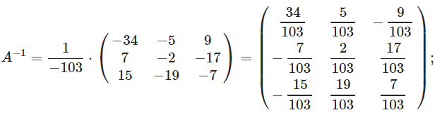
Since , then the system has a unique solution. Let's find all algebraic complements

, ,

Thus

Let's check

The inverse matrix was found correctly. From here, using the formula, we find the matrix of variables.

Comparing the values of the matrices, we get the answer: .

Cramer's method.

Let a system of linear equations with unknowns be given

and , i.e. the system has a unique solution. Let us write the solution of the system in matrix form or

Let's denote

. . . . . . . . . . . . . . ,

Thus, we obtain formulas for finding the values of unknowns, which are called Cramer formulas.

Example 28. Solve the following system of linear equations using the Cramer method .

Solution. Let's find the determinant of the main matrix of the system

Since , then the system has a unique solution.

Let's find the remaining determinants for Cramer's formulas

Using Cramer's formulas we find the values of the variables

Gauss method.

The method consists of sequential elimination of variables.

Let a system of linear equations with unknowns be given.

The Gaussian solution process consists of two stages:

At the first stage, the extended matrix of the system is reduced, using elementary transformations, to a stepwise form

where , to which the system corresponds

After this the variables are considered free and are transferred to the right side in each equation.

At the second stage, the variable is expressed from the last equation, and the resulting value is substituted into the equation. From this equation

the variable is expressed. This process continues until the first equation. The result is an expression of the main variables through free variables .

Example 29. Solve the following system using the Gauss method

Solution. Let's write out the extended matrix of the system and bring it to stepwise form

Because greater than the number of unknowns, then the system is consistent and has an infinite number of solutions. Let's write the system for the step matrix

The determinant of the extended matrix of this system, composed of the first three columns, is not equal to zero, so we consider it to be basic. Variables

They will be basic and the variable will be free. Let us move it in all equations to the left side

From the last equation we express

Substituting this value into the penultimate second equation, we get

where . Substituting the values of the variables and into the first equation, we find . Let's write the answer in the following form

Solving systems of linear algebraic equations is one of the main problems of linear algebra. This problem has important applied significance in solving scientific and technical problems; in addition, it is auxiliary in the implementation of many algorithms in computational mathematics, mathematical physics, and processing the results of experimental research.

A system of linear algebraic equations is called a system of equations of the form: (1)

Where – unknown; - free members.

Solving a system of equations(1) call any set of numbers that, when placed in system (1) in place of the unknowns converts all equations of the system into correct numerical equalities.

The system of equations is called joint, if it has at least one solution, and incompatible, if it has no solutions.

The simultaneous system of equations is called certain, if it has one unique solution, and uncertain, if it has at least two different solutions.

The two systems of equations are called equivalent or equivalent, if they have the same set of solutions.

System (1) is called homogeneous, if the free terms are zero:

A homogeneous system is always consistent - it has a solution (perhaps not the only one).

If in system (1), then we have the system n linear equations with n unknown: where – unknown; – coefficients for unknowns, - free members.

A linear system may have a single solution, infinitely many solutions, or no solution at all.

Consider a system of two linear equations with two unknowns

If then the system has a unique solution;

if then the system has no solutions;

if then the system has an infinite number of solutions.

Example. The system has a unique solution to a pair of numbers

The system has an infinite number of solutions. For example, solutions to a given system are pairs of numbers, etc.

The system has no solutions, since the difference of two numbers cannot take two different values.

Definition. Second order determinant called an expression of the form:

The determinant is designated by the symbol D.

Numbers A 11, …, A 22 are called elements of the determinant.

Diagonal formed by elements A 11 ; A 22 are called main diagonal formed by elements A 12 ; A 21 − side

Thus, the second-order determinant is equal to the difference between the products of the elements of the main and secondary diagonals.

Note that the answer is a number.

Example. Let's calculate the determinants:

Consider a system of two linear equations with two unknowns: where X 1, X 2 – unknown; A 11 , …, A 22 – coefficients for unknowns, b 1 , b 2 – free members.

If a system of two equations with two unknowns has a unique solution, then it can be found using second-order determinants.

Definition. A determinant made up of coefficients for unknowns is called system determinant: D= .

The columns of the determinant D contain the coefficients, respectively, for X 1 and at , X 2. Let's introduce two additional qualifier, which are obtained from the determinant of the system by replacing one of the columns with a column of free terms: D 1 = D 2 = .

Theorem 14(Kramer, for the case n=2). If the determinant D of the system is different from zero (D¹0), then the system has a unique solution, which is found using the formulas:

These formulas are called Cramer's formulas.

Example. Let's solve the system using Cramer's rule:

Solution. Let's find the numbers

Answer.

Definition. Third order determinant called an expression of the form:

Elements A 11; A 22 ; A 33 – form the main diagonal.

Numbers A 13; A 22 ; A 31 – form a side diagonal.

The entry with a plus includes: the product of elements on the main diagonal, the remaining two terms are the product of elements located at the vertices of triangles with bases parallel to the main diagonal. The minus terms are formed according to the same scheme with respect to the secondary diagonal.

Example. Let's calculate the determinants:

Consider a system of three linear equations with three unknowns: where – unknown; – coefficients for unknowns, - free members.

In the case of a unique solution, a system of 3 linear equations with three unknowns can be solved using 3rd order determinants.

The determinant of system D has the form:

Let us introduce three additional determinants:

Theorem 15(Kramer, for the case n=3). If the determinant D of the system is different from zero, then the system has a unique solution, which is found using Cramer’s formulas:

Example. Let's solve the system using Cramer's rule.

Solution. Let's find the numbers

Let's use Cramer's formulas and find the solution to the original system:

Answer.

Note that Cramer's theorem is applicable when the number of equations is equal to the number of unknowns and when the determinant of the system D is nonzero.

If the determinant of the system is equal to zero, then in this case the system can either have no solutions or have an infinite number of solutions. These cases are studied separately.

Let us note only one case. If the determinant of the system is equal to zero (D=0), and at least one of the additional determinants is different from zero, then the system has no solutions, that is, it is inconsistent.

Cramer's theorem can be generalized to the system n linear equations with n unknown: where – unknown; – coefficients for unknowns, - free members.

If the determinant of a system of linear equations with unknowns, then the only solution to the system is found using Cramer’s formulas:

An additional determinant is obtained from the determinant D if it contains a column of coefficients for the unknown x i replace with a column of free members.

Note that the determinants D, D 1 , … , D n have order n.

Gauss method for solving systems of linear equations

One of the most common methods for solving systems of linear algebraic equations is the method of sequential elimination of unknowns −Gauss method. This method is a generalization of the substitution method and consists of sequentially eliminating unknowns until one equation with one unknown remains.

The method is based on some transformations of a system of linear equations, which results in a system equivalent to the original system. The method algorithm consists of two stages.

The first stage is called straight ahead Gauss method. It consists of sequentially eliminating unknowns from equations. To do this, in the first step, divide the first equation of the system by (otherwise, rearrange the equations of the system). They denote the coefficients of the resulting reduced equation, multiply it by the coefficient and subtract it from the second equation of the system, thereby eliminating it from the second equation (zeroing the coefficient).

Do the same with the remaining equations and obtain a new system, in all equations of which, starting from the second, the coefficients for , contain only zeros. Obviously, the resulting new system will be equivalent to the original system.

If the new coefficients, for , are not all equal to zero, they can be excluded in the same way from the third and subsequent equations. Continuing this operation for the following unknowns, the system is brought to the so-called triangular form:

Here the symbols indicate the numerical coefficients and free terms that have changed as a result of transformations.

From the last equation of the system, the remaining unknowns are determined in a unique way, and then by sequential substitution.

Comment. Sometimes, as a result of transformations, in any of the equations all the coefficients and the right-hand side turn to zero, that is, the equation turns into the identity 0=0. By eliminating such an equation from the system, the number of equations is reduced compared to the number of unknowns. Such a system cannot have a single solution.

If, in the process of applying the Gauss method, any equation turns into an equality of the form 0 = 1 (the coefficients for the unknowns turn to 0, and the right-hand side takes on a non-zero value), then the original system has no solution, since such an equality is false for any values unknown.

Consider a system of three linear equations with three unknowns:

Where – unknown; – coefficients for unknowns, - free members. , substituting what was found

Solution. Applying the Gaussian method to this system, we obtain

Where does the last equality fail for any values of the unknowns, therefore, the system has no solution.

Answer. The system has no solutions.

Note that the previously discussed Cramer method can be used to solve only those systems in which the number of equations coincides with the number of unknowns, and the determinant of the system must be non-zero. The Gauss method is more universal and suitable for systems with any number of equations.

A system of m linear equations with n unknowns called a system of the form

Where a ij And b i (i=1,…,m; b=1,…,n) are some known numbers, and x 1 ,…,x n– unknown. In the designation of coefficients a ij first index i denotes the equation number, and the second j– the number of the unknown at which this coefficient stands.

We will write the coefficients for the unknowns in the form of a matrix , which we'll call matrix of the system.

The numbers on the right side of the equations are b 1 ,…,b m are called free members.

Totality n numbers c 1 ,…,c n called decision of a given system, if each equation of the system becomes an equality after substituting numbers into it c 1 ,…,c n instead of the corresponding unknowns x 1 ,…,x n.

Our task will be to find solutions to the system. In this case, three situations may arise:

A system of linear equations that has at least one solution is called joint. Otherwise, i.e. if the system has no solutions, then it is called incompatible.

Let's consider ways to find solutions to the system.

MATRIX METHOD FOR SOLVING SYSTEMS OF LINEAR EQUATIONS

Matrices make it possible to briefly write down a system of linear equations. Let a system of 3 equations with three unknowns be given:

Consider the system matrix and matrices columns of unknown and free terms

Let's find the work

those. as a result of the product, we obtain the left-hand sides of the equations of this system. Then, using the definition of matrix equality, this system can be written in the form

or shorter A∙X=B.

Here are the matrices A And B are known, and the matrix X unknown. It is necessary to find it, because... its elements are the solution to this system. This equation is called matrix equation.

Let the matrix determinant be different from zero | A| ≠ 0. Then the matrix equation is solved as follows. Multiply both sides of the equation on the left by the matrix A-1, inverse of the matrix A: . Since A -1 A = E And E∙X = X, then we obtain a solution to the matrix equation in the form X = A -1 B .

Note that since the inverse matrix can only be found for square matrices, the matrix method can only solve those systems in which the number of equations coincides with the number of unknowns. However, matrix recording of the system is also possible in the case when the number of equations is not equal to the number of unknowns, then the matrix A will not be square and therefore it is impossible to find a solution to the system in the form X = A -1 B.

Examples. Solve systems of equations.

CRAMER'S RULE

Consider a system of 3 linear equations with three unknowns:

Third-order determinant corresponding to the system matrix, i.e. composed of coefficients for unknowns,

called determinant of the system.

Let's compose three more determinants as follows: replace sequentially 1, 2 and 3 columns in the determinant D with a column of free terms

Then we can prove the following result.

Theorem (Cramer's rule). If the determinant of the system Δ ≠ 0, then the system under consideration has one and only one solution, and

Proof. So, let's consider a system of 3 equations with three unknowns. Let's multiply the 1st equation of the system by the algebraic complement A 11 element a 11, 2nd equation – on A 21 and 3rd – on A 31:

Let's add these equations:

Let's look at each of the brackets and the right side of this equation. By the theorem on the expansion of the determinant in elements of the 1st column

Similarly, it can be shown that and .

Finally, it is easy to notice that

Thus, we obtain the equality: .

Hence, .

The equalities and are derived similarly, from which the statement of the theorem follows.

Thus, we note that if the determinant of the system Δ ≠ 0, then the system has a unique solution and vice versa. If the determinant of the system is equal to zero, then the system either has an infinite number of solutions or has no solutions, i.e. incompatible.

Examples. Solve system of equations

GAUSS METHOD

The previously discussed methods can be used to solve only those systems in which the number of equations coincides with the number of unknowns, and the determinant of the system must be different from zero. The Gauss method is more universal and suitable for systems with any number of equations. It consists in sequentially eliminating unknowns from the equations of the system.

Consider again a system of three equations with three unknowns:

We will leave the first equation unchanged, and from the 2nd and 3rd we will exclude the terms containing x 1. To do this, divide the second equation by A 21 and multiply by – A 11, and then add it to the 1st equation. Similarly, we divide the third equation by A 31 and multiply by – A 11, and then add it with the first one. As a result, the original system will take the form:

Now from the last equation we eliminate the term containing x 2. To do this, divide the third equation by, multiply by and add with the second. Then we will have a system of equations: